Demo 2): Handling 3-dimensional fields

In this demo, you’ll learn the intricacies of how to handle and especially how to plot 3-dimensional fields, the specific pitfalls during plotting and how to avoid them.

Import:

import empyre as emp
import logging
logger = logging.getLogger()
logger.setLevel(logging.WARNING)

Create a 3D vortex

Similar to the first demo, we create a vortex distribution and the shape of a disc, which we’ll combine to generate a Field object (note that you can also use compound assignment operators like *=). This time, however, we generate a 3D distribution by using a shape of (32, 32, 32) for the dimension.

field = emp.fields.create_vector_vortex(dim=(32, 32, 32), core_r=3, oop_r=5)
field *= emp.fields.create_shape_disc(dim=(32, 32, 32), radius=10)

How to plot 3D distributions

If you try to use:

emp.vis.colorvec(field)

for plotting, you’ll get an error, telling you that you can only plot 2 dimensions (which makes sense for all 2D matplotlib plots). Instead of plotting the whole 3D volume, we can instead plot slices of it by using indices with the usual numpy bracket notation on our Field objects. Let’s try to plot a central slice along the z-direction. Note that the field_slice_z object is only two-dimensional with shape (32, 32)!

field_slice_z = field[15, ...]
emp.vis.colorvec(field_slice_z)
print(field)
print(field_slice_z)

Field(dim=(32, 32, 32), scale=(1.0, 1.0, 1.0), vector=True, ncomp=3)
Field(dim=(32, 32), scale=(1.0, 1.0), vector=True, ncomp=3)

Slices along other directions

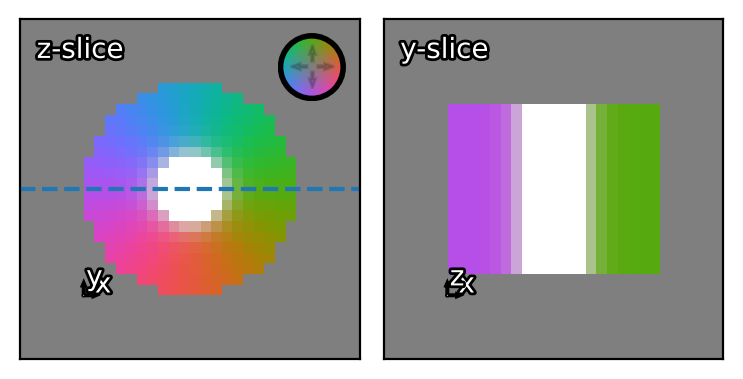
Next, let’s slice along the y-direction of the 3D volume (let’s again take a central slice through the volume) and compare the two slices. The dashed line in the left image shows, where the slice in the right image lies. You’ll notice that the color encoding in both images corresponds to the 3D directions of the vectors in our original 3D volume. This is due to the fact that our 2D slice still has information about the 3 components of the vector field. Furthermore, we’ll use some more decoration functions of vis, which should be self explanatory.

fig, axes = emp.vis.new(1, 2)
field_slice_y = field[:, 15, :]
emp.vis.colorvec(field_slice_z, axis=axes[0])
emp.vis.colorwheel(axis=axes[0])
emp.vis.annotate('z-slice', axis=axes[0])
emp.vis.coords(coords=('x', 'y'), axis=axes[0])
axes[0].axhline(y=16, linestyle='--')
emp.vis.colorvec(field_slice_y, axis=axes[1])
emp.vis.annotate('y-slice', axis=axes[1])
emp.vis.coords(coords=('x', 'z'), axis=axes[1])
print(field)
print(field_slice_y)

Field(dim=(32, 32, 32), scale=(1.0, 1.0, 1.0), vector=True, ncomp=3)
Field(dim=(32, 32), scale=(1.0, 1.0), vector=True, ncomp=3)

Quiver and its ambiguity in 3D

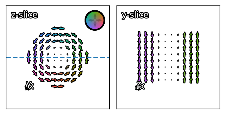
Let’s try the exact same plot with quiver instead of colorvec now. Note that we use the color_angles=True mode, which let’s us color the insides of the arrows the same way colorvec would. While the z-slice works finde, the y-slice may show the right colors, but the direction of the arrows are wrong. This is due to the fact that colorvec takes the information about all three vector components into account for coloring the pixels. This 3D color information is the same, however you slice the 3D volume (the vortex core will always point in positive z-direction, corresponding to white coloration). The arrows plotted by quiver, however have to be adapted to the current slicing plane and therefore need information about what this plane is! Note that field_slice_y has the shape (32, 32) and therefore is only 2-dimensional. quiver does not know how to assign the 3 vector components correctly to only 2 dimensions. To solve this ambiguity, quiver will only take the first two components, which erroneously interprets the slice as an x-y-plane. quiver will, however, warn the user about ambiguous assignments like this, if the number of vector components is larger than the number of dimensions.

fig, axes = emp.vis.new(1, 2)
field_slice_y = field[:, 15, :]
emp.vis.quiver(field_slice_z, color_angles=True, axis=axes[0])
emp.vis.colorwheel(axis=axes[0])
emp.vis.annotate('z-slice', axis=axes[0])
emp.vis.coords(coords=('x', 'y'), axis=axes[0])
axes[0].axhline(y=16, linestyle='--')
emp.vis.quiver(field_slice_y, color_angles=True, axis=axes[1])
emp.vis.annotate('y-slice', axis=axes[1])
emp.vis.coords(coords=('x', 'z'), axis=axes[1])
print(field)
print(field_slice_y)

c:\users\weber\documents\libertem\empyre\src\empyre\vis\plot2d.py:309: UserWarning: Assignment of vector components to dimensions is ambiguous!`ncomp` (3) should match `len(dim)` (2)!If you want to plot a slice of a 3D volume, make sure to use `from:to` notation!
  warnings.warn('Assignment of vector components to dimensions is ambiguous!'
c:\users\weber\documents\libertem\empyre\src\empyre\vis\plot2d.py:309: UserWarning: Assignment of vector components to dimensions is ambiguous!`ncomp` (3) should match `len(dim)` (2)!If you want to plot a slice of a 3D volume, make sure to use `from:to` notation!
  warnings.warn('Assignment of vector components to dimensions is ambiguous!'

Field(dim=(32, 32, 32), scale=(1.0, 1.0, 1.0), vector=True, ncomp=3)
Field(dim=(32, 32), scale=(1.0, 1.0), vector=True, ncomp=3)

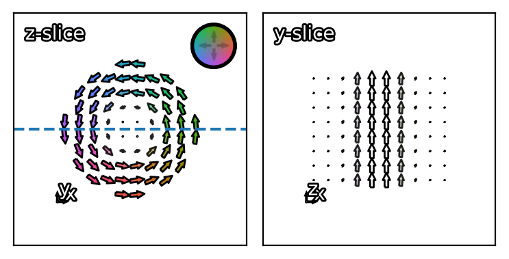
How to correctly use quiver in 3D

We can solve the ambiguity, by providing quiver with the information about which slice we really want to show. This can be done by slicing differently. Instead of using a single number to specify the slice in the y-direction, we use a slicing object (notation 15:16 in the example, or to:from in general). This way, the resulting field object will retain its 3-dimensional shape, but with a length of 1 along the slicing axis (here: (32, 1, 32)). In general, all 2D plotting routines can handle higher dimensional slices, as long as you can “squeeze” the fields to 2D by discarding dimensions of size 1. This is exaclty what is done in quiver, as well, but by providing the info about which axes are squeezed at the start of the function, quiver can now which vector components it should take to correctly plot the slice that the user wanted to plot. Note how in this example, the arrows in the vortex core are correctly pointing in positive z-direction (and are colored correctly, as well).#

fig, axes = emp.vis.new(1, 2)
field_slice_z_correct = field[15:16, ...]
field_slice_y_correct = field[:, 15:16, :]
emp.vis.quiver(field_slice_z_correct, color_angles=True, axis=axes[0])
emp.vis.colorwheel(axis=axes[0])
emp.vis.annotate('z-slice', axis=axes[0])
emp.vis.coords(coords=('x', 'y'), axis=axes[0])
axes[0].axhline(y=16, linestyle='--')
emp.vis.quiver(field_slice_y_correct, color_angles=True, axis=axes[1])
emp.vis.annotate('y-slice', axis=axes[1])
emp.vis.coords(coords=('x', 'z'), axis=axes[1])
print(field)
print(field_slice_y)
print(field_slice_y_correct)

Field(dim=(32, 32, 32), scale=(1.0, 1.0, 1.0), vector=True, ncomp=3)
Field(dim=(32, 32), scale=(1.0, 1.0), vector=True, ncomp=3)
Field(dim=(32, 1, 32), scale=(1.0, 1.0, 1.0), vector=True, ncomp=3)

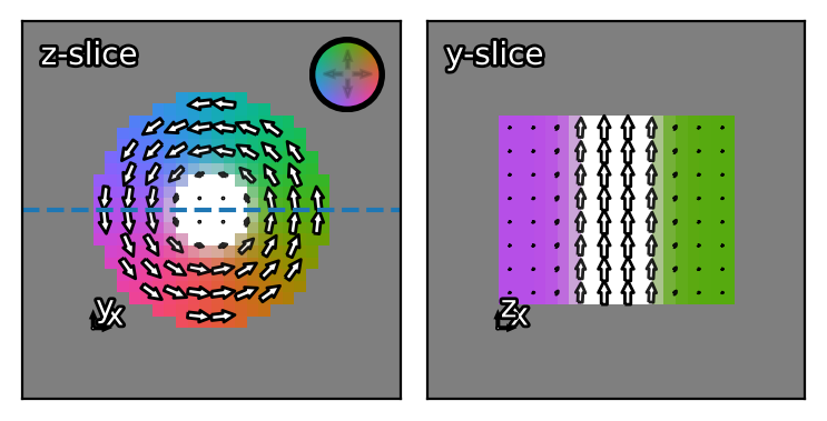
Combined plot

Let’s show colorvec and quiver in combination to generate a nice plot. Note that the points in the y-slice image (purple and green background) correspond to arrows in positive and negative y-direction (compare with the z-slice image) and are therefore out-of-plane for this specific slice.

fig, axes = emp.vis.new(1, 2)
emp.vis.colorvec(field_slice_z_correct, axis=axes[0])
emp.vis.quiver(field_slice_z_correct, axis=axes[0])
emp.vis.colorwheel(axis=axes[0])
emp.vis.annotate('z-slice', axis=axes[0])
emp.vis.coords(coords=('x', 'y'), axis=axes[0])
axes[0].axhline(y=16, linestyle='--')
emp.vis.colorvec(field_slice_y_correct, axis=axes[1])
emp.vis.quiver(field_slice_y_correct, axis=axes[1])
emp.vis.annotate('y-slice', axis=axes[1])
emp.vis.coords(coords=('x', 'z'), axis=axes[1])

('x', 'z')

Conclusion

This demo showed you how to correctly slice higher dimensional Field objects to utilize the 2D plot functions. In the next demo, we’ll see how we can load experimental data and how to use the many manipulation and transformation tools, that come with the Field class.