Demo 1): First steps and the Field class

In this first demo notebook, you’ll learn how to import the empyre package and how to utilize the Field class, which can contain multidimensional vector and scalar fields and is core to many functions of empyre. If you haven’t already, please visit the documentation to see how to install empyre.

Import:

First import empyre, we recommend to use the abbreviation emp. We’ll numpy as well.

import empyre as emp
import numpy as np

Represent your data with the ‘Field’ class

A Field object is a container for multi-dimensional vector or scalar fields, each Field has three parameters:

• data: Your underlying data, e.g. as a numpy array.

• scale: The axis scaling along each axis, given as a tuple. scale can be a given as a single number during construction of the Field object, which assumes that the scale is the same for all axes.

• vector: Determines if the field is a scalar field (vector=False, which is the default) or a vector field (vector=True). Please note that, if vector=True, the last axis of data is interpreted as the dimension of the vector components. The component dimension is the last one, so that the Field class can be indexed similarily to numpy arrays. This way, indexing a field with just spatial indices (by dropping the trailing component dimension) will work on scalar and vector fields at the same time. Most functions of Field are designed to work on both vector and scalar fields, as well.

We’ll start with a 2D scalar and a 2D vector field. You’ll find the base Field class in the fields submodule. Note that you can print fields to get a short summary about their parameters.

scalar_data = np.zeros((16, 16))
scalar_field = emp.fields.Field(data=scalar_data, scale=1, vector=False)
print(scalar_field)

vector_data = np.zeros((16, 16, 3))
vector_field = emp.fields.Field(data=vector_data, scale=1, vector=True)
print(vector_field)

Field(dim=(16, 16), scale=(1.0, 1.0), vector=False)
Field(dim=(16, 16), scale=(1.0, 1.0), vector=True, ncomp=3)

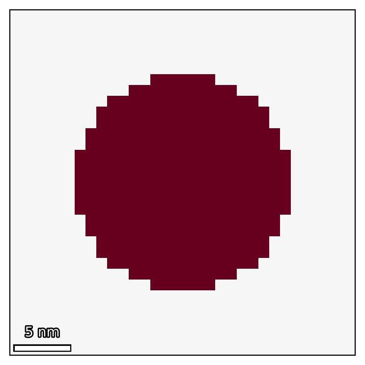
## Create more interesting fields with create_... functions The two fields created before are empty and not very interesting. The fields submodule has a few alternate constructor functions to generate shapes and vector fields in particular. Let’s look at the shapes submodule first, whose documentation can be found here (Note that all functions can be directly accessed via emp.fields.create_..., no need to access shapes directly). A simple example is the disc shape:

field_disc = emp.fields.create_shape_disc(dim=(32, 32), radius=10)
print(field_disc)

Field(dim=(32, 32), scale=(1.0, 1.0), vector=False)

## Visualize fields with the ‘vis’ subpackage The vis subpackage is used to visualize field objects. Its interface mirrors that of matplotlib and should be easy to learn if you are familiar with the latter. You can find the documentation here. Usually, scalar fields can be visualised with the imshow function (additional kwargs will be forwarded to the underlying matplotlib function, a behaviour shared by almost all 2D plot functions in vis):

emp.vis.imshow(field_disc)

c:\users\weber\documents\libertem\empyre\src\empyre\vis\plot2d.py:79: MatplotlibDeprecationWarning:
The DivergingNorm class was deprecated in Matplotlib 3.2 and will be removed two minor releases later. Use TwoSlopeNorm instead.
  kwargs.setdefault('norm', DivergingNorm(0))  # Diverging colormap should have zero at the symmetry point!

<matplotlib.image.AxesImage at 0x20a9b3d09e8>

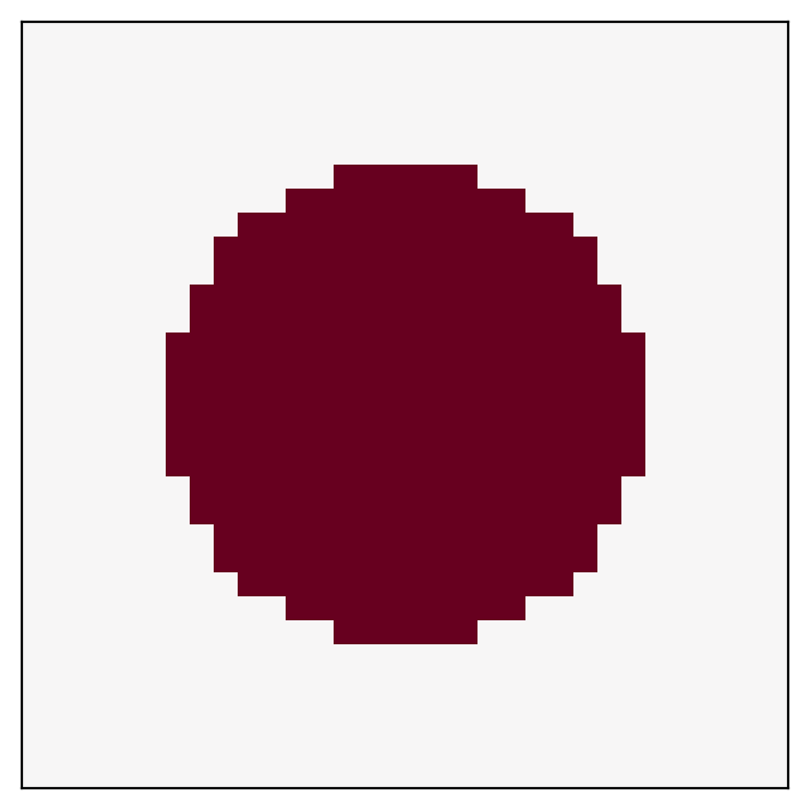
## Some vis basics The vis package has a lot of decorators that you can use to enhance your plots, you can find the documentation here. To apply them to a plot, just use the commands in the lines following a plot command. To generate a new plot, use the vis.new() function. If you are in a Jupyter notebook, like here, you don’t need new at the beginning of each cell, but new has some other neat features (like returning a grid of subplots) that could be useful for your specific case. Furthermore, empyre uses custom matplotlib stylesheets for ‘images’ and ‘plots’, respectively, which you can explicitely set in the new function with the mode parameter. For publications, new can specify the exact size of your plots according to your LaTeX document and save them afterwards with the savefig function. See here for more info on all of those features. empyre provides mainly plotting routines for images, but you can mix and match with matplotlib routines, for plots.

emp.vis.new(mode='image')  # Not necessary here, just for clarity, 'image' is the default!
emp.vis.imshow(field_disc)
emp.vis.scalebar()
# Create a new figure with two plots
fig, axes = emp.vis.new(nrows=1, ncols=2, aspect=0.3, mode='plot')
x = np.arange(10)
axes[0].plot(x, np.random.rand(10))
axes[1].plot(x, np.random.rand(10))

c:\users\weber\documents\libertem\empyre\src\empyre\vis\plot2d.py:79: MatplotlibDeprecationWarning:
The DivergingNorm class was deprecated in Matplotlib 3.2 and will be removed two minor releases later. Use TwoSlopeNorm instead.
  kwargs.setdefault('norm', DivergingNorm(0))  # Diverging colormap should have zero at the symmetry point!

[<matplotlib.lines.Line2D at 0x20a9daf0198>]